Keras: multi-label classification with ImageDataGenerator

This post was originally published in the GoDataDriven blog

Multi-label classification is a useful functionality of deep neural networks. I recently added this functionality into Keras' ImageDataGenerator in order to train on data that does not fit into memory. This blog post shows the functionality and runs over a complete example using the VOC2012 dataset.

Shut up and show me the code!

Images taken in the wild are extremely complex. In order to really "understand" an image there are many factors that play a role, like the amount of objects in the image, their dynamics, the relation between frames, the positions of the objects, etc. In order to make AI capable of understanding images in the wild as we do, we must empower AI with all those capabilities. This empowerment may come in different ways, such like multi-class classification, multi-label classification, object detection (bounding boxes), segmentation, pose estimation, optical flow, etc.

After a small discussion with collaborators of the keras-preprocessing package we decided to start empowering Keras users with some of these use cases through the known ImageDataGenerator class. In particular, thanks to the flexibility of the DataFrameIterator class added by @Vijayabhaskar this should be possible.

Then, during our last GDD Friday at GoDataDriven I decided to go ahead and start adding the multi-class classification use case.¹ The end result was this PR.

But first... What is multi-label classification?

Not to be confused with multi-class classification, in a multi-label problem some observations can be associated with 2 or more classes.

NOTE

This functionality has just been released in PyPI yesterday in the keras-preprocessing 1.0.6 version. You can update keras to have the newest version by:

pip install -U keras

Multi-class classification in 3 steps

In this part will quickly demonstrate the use of ImageDataGenerator for multi-class classification.

1. Image metadata to pandas dataframe

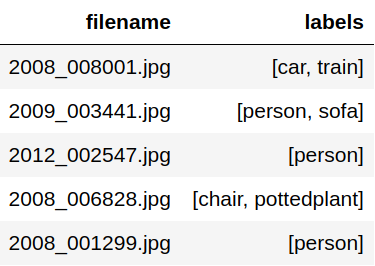
Ingest the metadata of the multi-class problem into a pandas dataframe. The labels for each observation should be in a list or tuple. The filenames of the images can be ingested into the dataframe in two ways as shown in the image below.

• Relative paths: If you only state the filenames of the images you will have to use the directory argument later on when calling the method flow_from_dataframe.

• Absolute paths: In this case you can ditch the directory argument. ²

2. Instantiate DataFrameIterator

Create the generator of the images batches. This is done by instantiating DataFrameIterator via the flow_from_dataframe method of ImageDataGenerator. Supposing we ingested the filenames as relative paths, the simplest instantantiation would look like this:³

from keras.preprocessing.image import ImageDataGenerator

img_iter = ImageDataGenerator().flow_from_dataframe(
    img_metadata_df,
    directory='/home/rodrigo/.keras/datasets',
    x_col='filename',
    y_col='labels',
    class_mode='categorical'
)

The actual logic of creating the batches and handling data augmentation is managed by the DataFrameIterator class. You can look up other available arguments in here.

3. Train the model

Train the model using the fit_generator method.⁴

model.fit_generator(img_iter)

This will yield batches directly from disk, allowing you to train on much more data than it can fit in your memory.

That's it!⁵

Rundown example with VOC2012

In this part I'll walk you through a multi-class classification problem step by step. The example will use the VOC2012 dataset which consist of ~17,000 images and 20 classes.

Just by looking at the images below you can quickly observe that this is a quite diverse and difficult dataset. Perfect! The closer to a real-life example the better.

Let's start by downloading the data into ~/.keras/datasets from here.

~/.keras/datasets/VOC2012
├── Annotations
│   ├── 2010_000002.xml
│   ├── 2010_000003.xml
│   ├── 2011_000002.xml
│   └── ...
├── ImageSets
│   ├── Action
│   ├── Layout
│   ├── Main
│   └── Segmentation
├── JPEGImages
│   ├── 2010_000002.jpg
│   ├── 2010_000003.jpg
│   ├── 2011_000002.jpg
│   └── ...
├── SegmentationClass
│   ├── 2010_000002.png
│   ├── 2010_000003.png
│   └── 2011_000003.png
└── SegmentationObject
    ├── 2010_000002.png
    ├── 2010_000003.png
    └── ...

We will use the Annotations directory to extract the images metadata. Each image can also have repeated associated labels, the argument unique_labels of the function below regulates if we keep repeated labels. We will not, trust me, the problem is hard enough.

import xml.etree.ElementTree as ET
from pathlib import Path

def xml_to_labels(xml_data, unique_labels):
    root = ET.XML(xml_data)
    labels = set() if unique_labels else []
    labels_add = labels.add if unique_labels else labels.append # speeds up method lookup
    for i, child in enumerate(root):
        if child.tag == 'filename':
            img_filename = child.text
        if child.tag == 'object':
            for subchild in child:
                if subchild.tag == 'name':
                    labels_add(subchild.text)
    return img_filename, list(labels)

def get_labels(annotations_dir, unique_labels=True):
    for annotation_file in annotations_dir.iterdir():
        with open(annotation_file) as f:
            yield xml_to_labels(f.read(), unique_labels)

annotations_dir = Path('~/.keras/datasets/VOC2012/Annotations').expanduser()
img_metadata = pd.DataFrame(get_labels(annotations_dir), columns=['filename', 'labels'])

After extraction we end up with a dataframe with relative paths as shown below.

The filenames are then relative to

images_dir = Path('~/.keras/datasets/VOC2012/JPEGImages').expanduser()

Scan the dataset

Let's now have a quick look at how the labels are distributed accross the dataset. These counts can be easily be computed with a Counter object.

from collections import Counter
labels_count = Counter(label for lbs in img_metadata['labels'] for label in lbs)

From here we can easily compute the class_weights for later use.

total_count = sum(labels_count.values())
class_weights = {cls: total_count / count for cls, count in labels_count.items()}

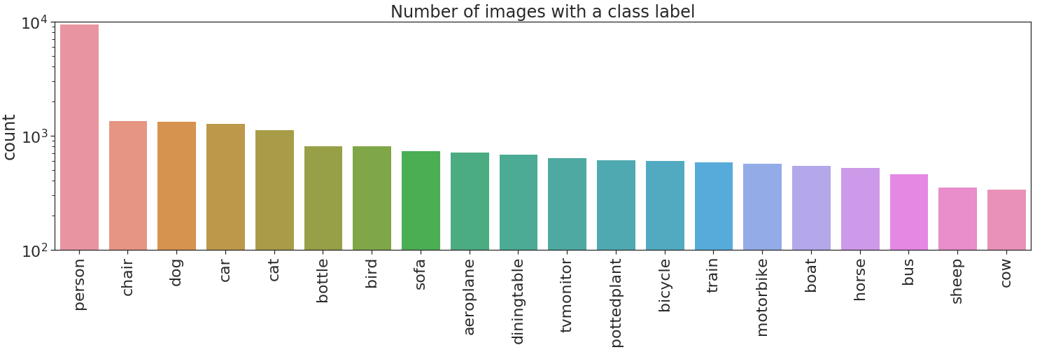
Let's now plot the labels count.

No bueno, no bueno at all! There are two types of imbalances in the dataset. Imbalance across different classes, and imbalance between positive and negative examples in some classes. The former imbalance type can produce overfitting to highly represented classes, person in this case. The latter imbalance type can produce that a class is always flagged as negative i.e. if cow will always be flagged negative this will yield a 97% accuracy on that class.

So what can we do about it?... pray. I won't go into detail but one way to counter the imbalances is with a combination of class weights and sample weights.⁶

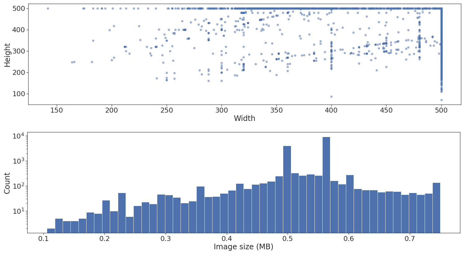
Next step is to look at the shape and size distribution across the different images.

As illustrated above, the dataset contains images of different heights and widths. I won't go into detail, but this is not really a problem if at the end of the feature extraction via convolutional layers a global pooling layer is applied. Unfortunately, there is another problem, when using flow_from_dataframe all images need to be standardized to the same width and height.⁷ This is specified via the target_size parameter.

The lower histogram plot is good to have because it can give us an approximate indication of the maximum batch and queue size our memory can fit when using the generator. In this example, I don't really use the plot though.

Training the model

First, we need to instantiate the ImageDataGenerator. I'll do this with a simple setup just normalizing the pixel values. I also included a validation split to use it for validation stats during training after each epoch.

img_gen = ImageDataGenerator(rescale=1/255, validation_split=0.2)

We can now create the training and validation DataFrameIterator by specifying subset as "training" or "validation" respectively. In the case of multi-label classification the class_mode should be "categorical" (the default value).

img_iter = img_gen.flow_from_dataframe(
    img_metadata,
    shuffle=True,
    directory=images_dir,
    x_col='filename',
    y_col='labels',
    class_mode='categorical',
    target_size=(128, 128),
    batch_size=20,
    subset='training'
)

img_iter_val = img_gen.flow_from_dataframe(
    img_metadata,
    shuffle=False,
    directory=images_dir,
    x_col='filename',
    y_col='labels',
    class_mode='categorical',
    target_size=(128, 128),
    batch_size=200,
    subset='validation'
)

I will use the ResNet50 pre-trained model in this example. I will replace the last fully connected layers of the network by an output layer with 20 neurons, one for each class.⁸ In addition, pay attention to the output activation function, I won't go into detail, but for multi-class classification the probability of each class should be independent, hence the use of the sigmoid function and not the softmax function which is used for multi-class problems.

base_model = ResNet50(
    include_top=False,
    weights='imagenet',
    input_shape=None,
    pooling='avg'
)
for layer in base_model.layers:
    layer.trainable = False

predictions = Dense(20, activation='sigmoid')(base_model.output)
model = Model(inputs=base_model.input, outputs=predictions)

Next we compile the model using "binary_crossentropy" loss. Why binary cross-entropy and not categorical cross-entropy you ask? well, again, I won't go into detail, but if you use categorical_crossentropy you are basically not penalizing for false positives (if you are more of a code person than a math person here you go).

model.compile(
    loss='binary_crossentropy',
    optimizer='adam'
)

NOTE: Even though I just said that for multi-label the math dictates sigmoid and binary cross-entropy, there are cases out there where softmax and categorical cross-entropy worked better. Like this one.

Train the model already! Not yet... patience, "lento pero seguro". Let's talk about metrics for a multi-label problem like this. I hope it is obvious that accuracy is not the way to go. Instead, let's use f1_score, recall_score and precision_score. There is a slight problem though, yes life is a bitch, these metrics were removed from the keras metrics with a good reason.

The correct way to implement these metrics is to write a callback function that calculates them at the end of each epoch over the validation data. Something like this:

from itertools import tee  # finally! I found something useful for it
from sklearn import metrics

class Metrics(Callback):
    def __init__(self, validation_generator, validation_steps, threshold=0.5):
        self.validation_generator = validation_generator
        self.validation_steps = validation_steps or len(validation_generator)
        self.threshold = threshold

    def on_train_begin(self, logs={}):
        self.val_f1_scores = []
        self.val_recalls = []
        self.val_precisions = []

    def on_epoch_end(self, epoch, logs={}):
        # duplicate generator to make sure y_true and y_pred are calculated from the same observations
        gen_1, gen_2 = tee(self.validation_generator)
        y_true = np.vstack(next(gen_1)[1] for _ in range(self.validation_steps)).astype('int')
        y_pred = (self.model.predict_generator(gen_2, steps=self.validation_steps) > self.threshold).astype('int')
        f1 = metrics.f1_score(y_true, y_pred, average='weighted')
        precision = metrics.precision_score(y_true, y_pred, average='weighted')
        recall = metrics.recall_score(y_true, y_pred, average='weighted')
        self.val_f1_scores.append(f1)
        self.val_recalls.append(recall)
        self.val_precisions.append(precision)
        print(f" - val_f1_score: {f1:.5f} - val_precision: {precision:.5f} - val_recall: {recall:.5f}")
        return

Finally! we are ready to train the model. FYI: I did little to no effort to optimize the model.

metrics = Metrics(img_iter_val, validation_steps=50)
history = model.fit_generator(
    img_iter,
    epochs=10,
    steps_per_epoch=250,
    class_weight=class_weights,
    callbacks=[metrics]
)

During the training time you should see validation metrics at the end of each epoch, something like this:

Epoch 10/10
250/250 [==============================] - 261s 1s/step - loss: 5.0277 - val_f1_score: 0.28546 - val_precision: 0.21283 - val_recall: 0.58719

If your memory melts during training reduce the batch_size, the target_size or the max_queue_size parameters.

Post-mortem investigation

In the case of a multi-class problem, it is already of big help to plot the confusion matrix, in that way we can identify very clearly where the model is "confusing" one class for another and address the problems directly. Due to the multi-label nature of the problem makes no sense to do the same. Instead a confusion matrix per class can be reviewed.⁹

This functionality is only in the development version of scikit-learn, you can get that version by

pip install git+https://www.github.com/scikit-learn/scikit-learn.git --upgrade

after that you should be able to

from sklearn.metrics import multilabel_confusion_matrix

I wrote a wrapper plot function plot_multiclass_confusion_matrix around multilabel_confusion_matrix, which you can find in the code. The output from it looks like this:

That's it folks! As you can see the model sucks. Your mission, should you choose to accept it...

Adios

I hope you found this blog post useful. I went through many concepts rather quickly but I think there are some valuable tips in there.

You can find the code here.

If you have any other questions just ping me on twitter @rragundez.