"I Pity the fool", Deep Learning style

This post was originally published in the GoDataDriven blog

With deep learning applications blossoming, it is important to understand what makes these models tick. Here I demonstrate, using simple and reproducible examples, how and why deep neural networks can be easily fooled. I also discuss potential solutions.

Several studies have been published on how to fool a deep neural network (DNN). The most famous study, which was published in 2015 used evolutionary algorithms or gradient ascent to produce the adversarial images.¹ A very recent study (October 2017) revealed that fooling a DNN could be achieved by changing a single pixel.² This subject seems fun and all but has substantial implications on current and future applications of deep learning. I believe that understanding what makes these models tick is extremely important to be able to develop robust deep learning applications (and avoid another event like random forest mania).³

A comprehensive and complete summary can be found in the When DNNs go wrong blog, which I recommend you to read.

All these amazing studies use state of the art deep learning techniques, which makes them (in my opinion) difficult to reproduce and to answer questions we might have as non-experts in this subject.

My intention in this blog is to bring the main concepts down to earth, to an easily reproducible setting where they are clear and actually visible. In addition, I hope this short blog can provide a better understanding of the limitations of discriminative models in general. The complete code used in this blog post can be found here.

Discriminative what?

Neural networks belong to the family of discriminative models, they model the dependence of an unobserved variable (target) based on observed input (features). In the language of probability this scenario is represented by the conditional probability and it is expressed as:

$$p(target|features)$$

it reads: the probability of the target given the features (e.g. the probability that it will rain based on yesterday's weather, temperature and pressure measurements).

Multinomial logistic regression models are also part of these discriminative models and they basically are a neural network without a hidden layer. Please don't be disappointed but I will start by demonstrating some concepts using multinomial logistic regression. Then I'll expand the concepts to a deep neural network.

Fooling multinomial logistic regression

As mentioned before a multinomial logistic regression can be seen as a neural network without a hidden layer. It models the probability of the target ($Y$) being a certain category ($c$), as a function ($F$) that depends on the linear combination of the features ($X=(X_1, X_2,...,X_N)$). We write this as

$$P(Y=c|X)=F(\theta_{c}^T\cdot X)$$

where $\theta_c$ are the coefficients of the linear combination for each category. The predicted class by the model is the one which gives the highest probability.

When the target $Y$ is binary, $F$ is taken to be some sigmoid function, the most common being the logistic function. When $Y$ is multiclass we commonly use $F$ as the softmax function.

Apart from the conceptual understanding of discriminative models, the linear combination of the features ($\theta_{c}^T\cdot X$) is what makes classification models vulnerable as I will demonstrate. In the own words of Master Jedi Goodfellow: "Linear behavior in high-dimensional spaces is sufficient to cause adversarial examples".⁴

Iris dataset

When I was thinking on how to do this blog post and actually visualize the concepts, I concluded I needed two things:

• A 2-dimensional feature space.
• A model with high accuracy on this space.

The 2-dimensional space because I wanted to generate plots which directly show the concepts. High accuracy because it's meaningless if I am able to fool a bad model.

Lucky for me, it turns out that a good accuracy can be obtained on the Iris dataset by just keeping two features: petal length and petal width.

Putting everything into shape this is how the data looks like

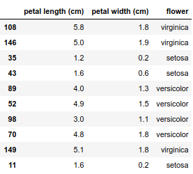
This dataset contains only 150 observations, I will fit the model to all the data using a cross-entropy loss function and a L2 regularization term. This is just a plug and play from the amazing scikit-learn.

model = LogisticRegression(max_iter=100, solver='lbfgs', multi_class='multinomial', penalty='l2')
model.fit(X=iris.loc[:, iris.columns != 'flower'], y=iris.flower)

The mean accuracy of the model is $96.6\%$. This score is based on the training data and can be misleading, even if I am using a regularization term I can still be overfitting.⁵

Let's now look at our predictions and at how our model is drawing the classification boundaries.

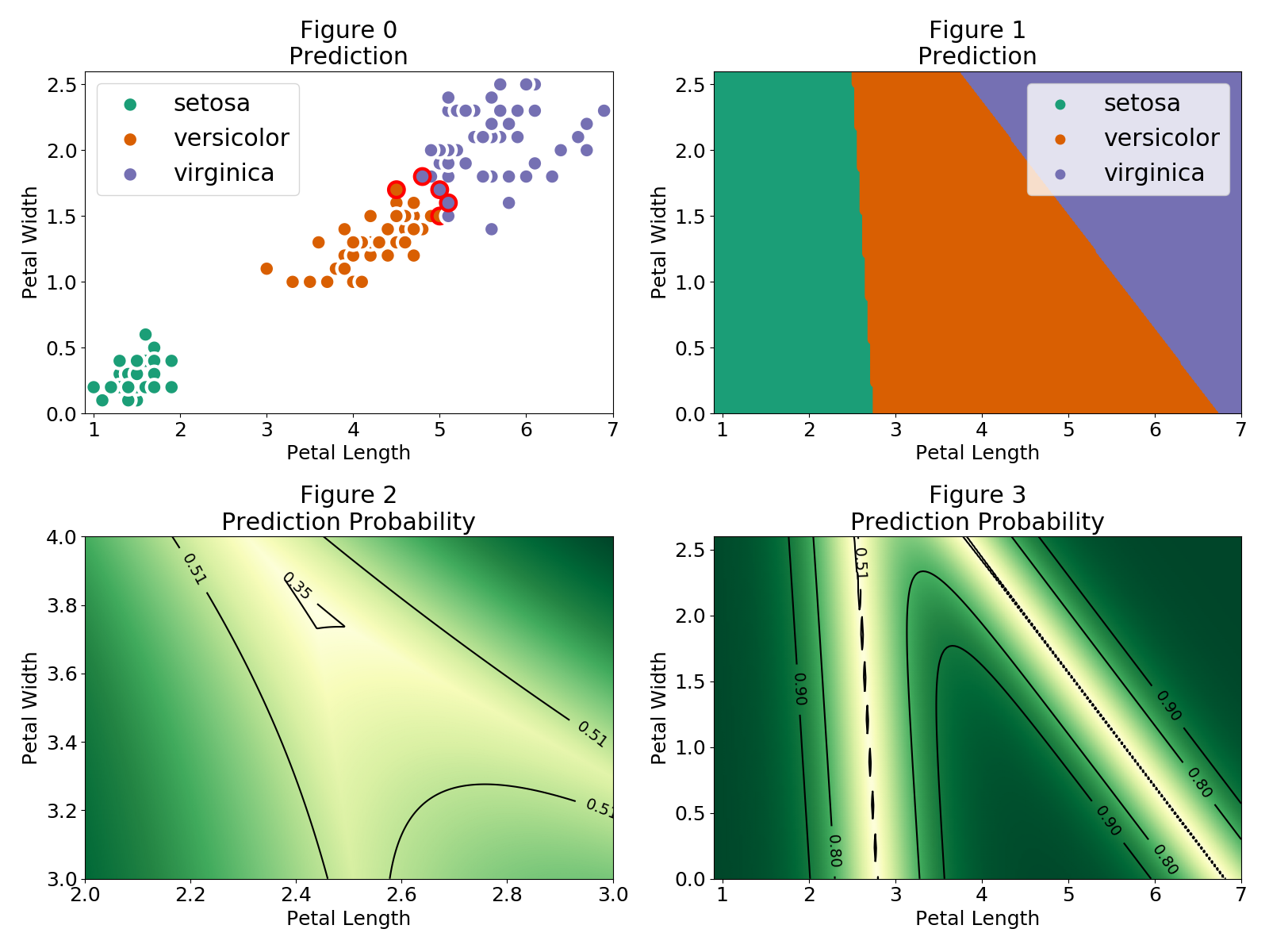
In Figure 0 the red outer circles indicate those observations that were wrongly classified. The setosa flowers are easily identified and there is a region where the versicolor and virginica observations are close together. In Figure 1 we can see the different regions for each flower category. The regions are separated by a linear boundary, this is a consequence of the linear combination model used $P(Y=c|X)=F(\theta_{c}^T\cdot X)$. As mentioned, in the case of a logistic regression (binary classification) $F$ is the logistic function

$$F(\theta_{c}^T\cdot X)=\frac{1}{1 + e^{-\theta_{c}^T\cdot X}}$$

and the classification boundary is given by $P(Y=c|X)=\frac{1}{2}$ when $\theta_{c}^T\cdot X=0$. If the features are in one dimension then the boundary will be a single value, for two features the boundary is a single line and for three features a plane and so on. In our multinomial case we use the softmax function

$$F(\theta_{c}^T\cdot X)=\frac{e^{\theta_{c}^T\cdot X}}{\Sigma_{i=1}^Ne^{\theta_{i}^T\cdot X}}$$

where the sum over $i$ in the denominator runs over all the possible classes of the target. In the regions where only two classes have a non-negligible probability the softmax function simplifies to the logistic function. Therefore the linear classification boundaries between two regions is given by the contour $P(Y=c|X)=\frac{1}{2}$ as shown in Figure 3. In addition, when none of the classes have a negligible probability the boundary approaches the contour $P(Y=c|X)=\frac{1}{3}$ where the uncertainty of our prediction is maximum. This region is illustrated in Figure 2.

A thing to note is that the regions extend to values which can be very far from the observations, which means we can grab a petal length of 1 and petal width of 4 and still be classified as a setosa. Even more, Figure 4 shows that even far away from our observations we can find regions with extremely high probability. We can even use a negative petal length!

Let's pick some points from Figure 4 and see if I am able to fool the multinomial logistic classifier:

• Point: (.1, 5)
  • Prediction: setosa
  • Probability: 0.998
• Point: (10, 10)
  • Prediction: virginica
  • Probability: 1.0
• Point: (5, -5)
  • Prediction: versicolor
  • Probability: 0.992

The three points give a high probability on the prediction but are not even remotely like the observations in our dataset.

Ok, now to the good stuff.

Fooling a Deep Neural Network

As I said before, in order for me to demonstrate the concepts and have a comprehensive visualization I need two things

• A 2-dimensional feature space.
• A model with high accuracy on this space.

In the case of a deep neural network it makes no sense to attack a problem with 2 features, as the intent of neural network is to throw a bunch of features as the input layer and let the hidden layers figure out and construct new features which are relevant to my classification problem. So my reasoning as how to solve my first requirement goes as follows:

1. Build a DNN where the last hidden layer has two units.
2. Then do the space analysis on the features from that layer.
3. Pick a point on that layer space which is far from the propagated observations but still is classified with a high probability.
4. Invert all the operations made from the input layer to that last hidden layer and apply them to my selected 2D point from step 3.

If I can perform those steps I should end with an input which is nothing like my observations but still is classified with high probability by the DNN, giving me an adversarial example.

MNIST

I chose the MNIST digits since it is a straight forward dataset to perform classification and it is complex enough to apply a DNN. I only take 4 classes, the numbers ${0, 1, 2, 3}$. The final dataset consists of a bit more than 28,000 observations with 28x28=784 features.

digits = fetch_mldata("MNIST original")
index = np.in1d(digits.target, [0, 1, 2, 3])
digits.data = digits.data[index]
digits.target = digits.target[index]

Number of observations: 28911
Nr. observations per class:
1.0    7877
3.0    7141
2.0    6990
0.0    6903

A sample view of our observations:

DNN configuration

The challenge here is to find the correct configuration such that the training of the DNN converges and has a good performance on the training set.

In addition, in order to be able to invert all the operations from the input layer to the last hidden layer then all functions applied must have an inverse. This means that if I decide to use any of the activation functions provided: logistic, tanh and relu, I need to keep track and impose restrictions on my nodes activation so that they are in the codomain of the activation function. This is not trivial and in my opinion does not add much to the concepts I'm trying to get across. Therefore I use the identity activation which can make the convergence a bit more tricky. ⁶

The final configuration of the DNN consists of:

• 3 hidden layers with sizes {50, 20, 2}.
• Identity activation function (no activation function).
• Stochastic gradient descent optimizer (sgd).
• Adaptive learning rate.

dnn_identity = MLPClassifier(
    hidden_layer_sizes=(50, 20, 2),
    activation='identity',
    solver='sgd',
    learning_rate = 'adaptive', learning_rate_init=.00005,
    random_state=21
)

The DNN achieved close to 95% accuracy and reached conversion quite nicely as shown in Figure 6. For comparison and for use in my arguments I built another DNN with an activation function $tanh$ using the Adam optimizer.

dnn_tanh = MLPClassifier(
    hidden_layer_sizes=(50, 20, 2),
    activation='tanh',
    solver='adam',
    learning_rate_init=.0001,
    random_state=21
)

The second DNN with the activation function achieved an accuracy of 98%, the loss curve in Figure 7 reveals that the training can be further improved but for now this is good enough.

Extract feature encoding from the last hidden layer

Once the model is trained we can retrieve the coefficients connecting all the layers. We use these coefficients to "manually" propagate our observations input up to the last hidden layer and then plot some of them in a 2D graph. This small function propagates the input layer up to a specified layer.

def propagate(input_layer, layer_nr, dnn, activation_function):
    """Obtain the activation values of any intermediate layer of the deep neural network."""
    layer = input_layer
    for intercepts, weights in zip(dnn.intercepts_[:layer_nr], dnn.coefs_[:layer_nr]):
        layer = activation_function(layer.dot(weights) + intercepts)
    return layer

hl_identity = propagate(digits.data, 3, dnn_identity, lambda x: x)
hl_tanh = propagate(digits.data, 3, dnn_tanh, np.tanh)

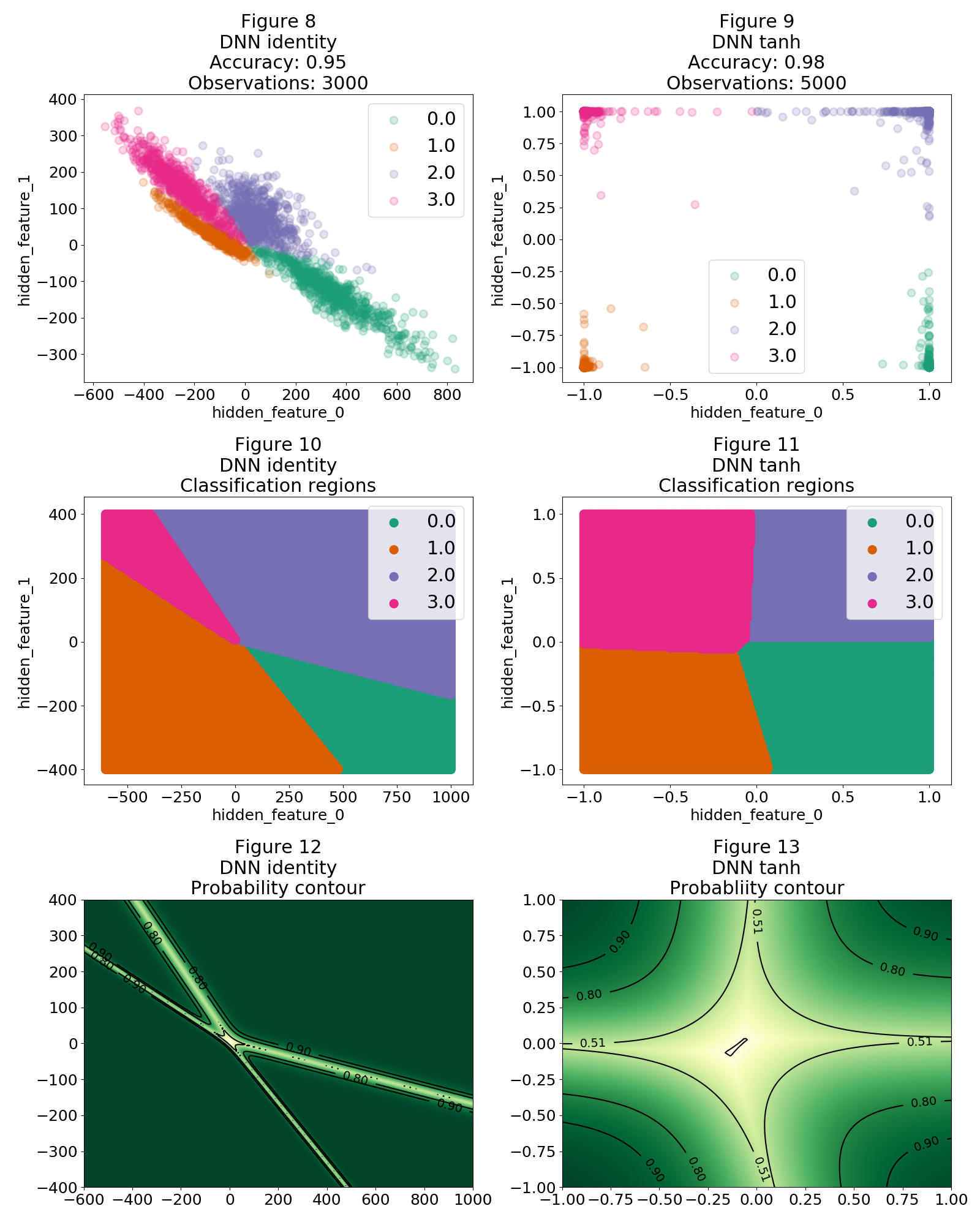
The representation of the observations under the encoding of the last 2D hidden layer is shown on Figure 8 and 9. The identity DNN, as shown in Figure 8, has encoded our observations by creating hidden features which separate them in the hidden layer dimensionality (2D in this case). The more sophisticated $tanh$ DNN achieves better performance because it is capable of coming up with hidden features which separate in a better way our observations as shown in Figure 9. Nevertheless Figures 10 and 11 reveal that in both cases linear classification boundaries are being constructed to separate our category regions. Similar to the multinomial logistic regression, this is caused by the dot product (linear Kernel) between the last hidden layer and the final weights which connect the hidden layer with the output layer. This means that these regions extend far away from where our observations lie, even more these regions have a high probability as shown in Figure 12 and 13.

So now the only thing to do is to grab a point from Figure 8 (for example: -200, 200), do all the inverse operations to bring back the encoding to the input layer and reshape the vector into an image which of course will look nothing like a $1$ but will be classified as a $1$ with very high probability by our DNN.

Brief tangent

Before proceeding I would like to have a more conceptual discussion regarding the implications of the arguments presented for figure 8 and 9. The DNN creates hidden features which separate our observations as best as possible. This means that such hidden features will concentrate on capturing differences between our classes. For example, let's say we want to classify dogs and horses⁷. According to our reasoning, will a feature that captures the amount of legs be created? I don't think so, because having such a feature doesn't add to the purpose of separating our classes. We can send a horse with 5 legs and this fact will not raise any flags on our DNN. I believe this is the underlying concept when we say that discriminative models do not capture the essence of the objects to be classified. Here is where generative models come to the rescue, they recently have shown amazing results by capturing the underlying "context" of the objects. In a probability framework they shift from modelling the conditional probability to model the joint probability.

Notice that the probability near the boundaries grows exponentially with the product $\theta_c\cdot X$ following the sigmoid function. This means that if we take an observation which lies close to a boundary, it takes a small perturbation to take it to another region. This is the principle behind the study of fooling a DNN with a single pixel change².

Finally notice that all our analysis is in a 2D space and as such the regions extend in a surface. In a 3D space these regions will become volumes, hence increasing the region size where adversarial examples can be found. Just like Master Jedi Goodfellow said: "Linear behavior in high-dimensional spaces is sufficient to cause adversarial examples" ³.

Pity the fool

A bit of linear algebra. Two consecutive layers can be described by a set of linear equations which in matrix notation can be represented by⁸:

$$L_{N}^i\times \Theta_{N\times M}=L_{M}^{i+1}$$

where $i$ is a certain layer number, $N$ and $M$ the number of units in the layer and $\Theta$ the coefficients representing the connections between layers. In our DNN each layer reduces in size, this means that $N>M$. In order to find the layer $i$ from the layer $i+1$ we need to find the inverse of $\Theta_{N\times M}$ and compute

$$L_{N}^i=L_{M}^{i+1}\times \Theta_{N\times M}^{-1}$$

The problem (of course) is that non-square matrices do not have an inverse. In the DNN context, what is happening is that we are losing information by compacting our observations in a lower dimensional space. This means there is no way to exactly trace back layers, simply because we don't have enough information. This does not mean that we cannot find a vector representing $L^i_N$ which satisfies $L_{N}^i\times \Theta_{N\times M}=L_{M}^{i+1}$ given the layer $L^{i+1}M$ and the coefficients $\Theta$, which means that such vector is not unique.

A solution for the layer $L_{N}^i$ can be derived using the pseudoinverse, in particular the Moore–Penrose inverse is adequate for our type of problem, and best of all it is implemented in Numpy!

Below I define a function which inverts the propagation from a hidden layer to the input layer with an identity activation function.⁹

def invert_propagation(hidden_layer, layer_nr, dnn):
    """Obtain the input layer from a hidden layer of a deep neural network"""
    layer = hidden_layer
    for intercepts, weights in zip(nn.intercepts_[layer_nr::-1], nn.coefs_[layer_nr::-1]):
        inv_weight = np.linalg.pinv(weights)
        layer = (layer - intercepts).dot(inv_weight)
    return layer

Finally, the moment of truth. I choose a nonsense value for each region by looking at Figures 10 and 12. In particular I choose:

• Region 0: (1200, -300)
• Region 1: (-500, 500)
• Region 2: (100,400)
• Region 3: (-1000, 900)

Now I invert the propagation for each point, obtain the input layer, reshape the input to a 28x28 image and show it together with the prediction from the DNN and the probability of such prediction.

def pity_the_fool(hidden_vector, dnn, ax):
    input_vector = invert_propagation(hidden_vector, 2, dnn_identity)
    ax.imshow(input_vector.reshape((28, 28)), cmap='gray')

    prediction = dnn.predict(input_vector.reshape(1, -1))[0]
    probability = np.max(dnn.predict_proba(input_vector.reshape(1, -1)))

    ax.set_title("Prediction: {:.0f}\n"
                 "Probability: {:.3f}\n"
                 "Hiden vector: {}"
                 .format(prediction, probability, hidden_vector))
    ax.axis('off')

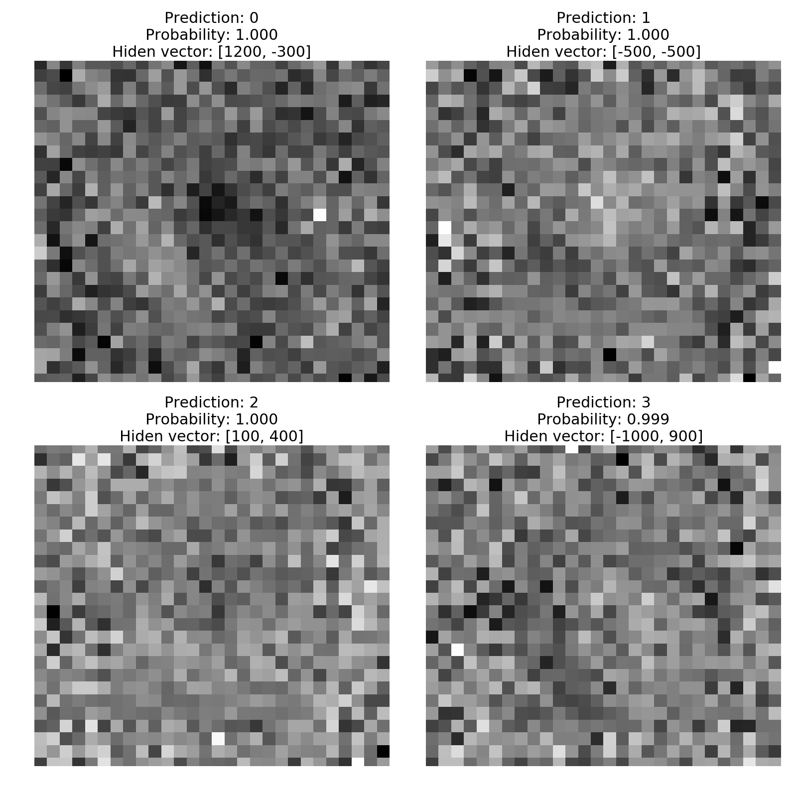
The figures above clearly show that I have managed to fool the DNN. It is like the DNN had some Mexican peyote or something. The labels are consistent with the regions we took the points from and are classified with almost 100% probability. There is no way a human eye can tell that those images are a 0, a 1, a 2 and a 3. Not even to tell that there are numbers.

Light at the end of the tunnel

I have stated that the main problem is the linear classification boundaries, is there a way we can avoid this? Well, I left a hint out there when I mentioned that the dot product presented is nothing more than a linear kernel. I will not go into the details of how the kernel trick works, but in summary it lets us perform dot products in higher dimensional spaces of our features without ever computing the new features in that high-dimensional space. If you never heard about it, it can be a bit of a weird thing. Just to mess more with your cerebro, if for example we were to use the Gaussian kernel, this is equal to performing calculations in an infinite high-dimensional space, yes infinite! ¹⁰

By using these kernels the model is not restricted to linear classification boundaries. Below I compare a support vector machine model (SVM) with a linear kernel and a Gaussian kernel using the iris dataset.

svm_linear = SVC(kernel='linear', probability=True)
svm_gaussian = SVC(kernel='rbf', probability=True)

Both SVM models obtain an accuracy of $\approx 96.6%$.

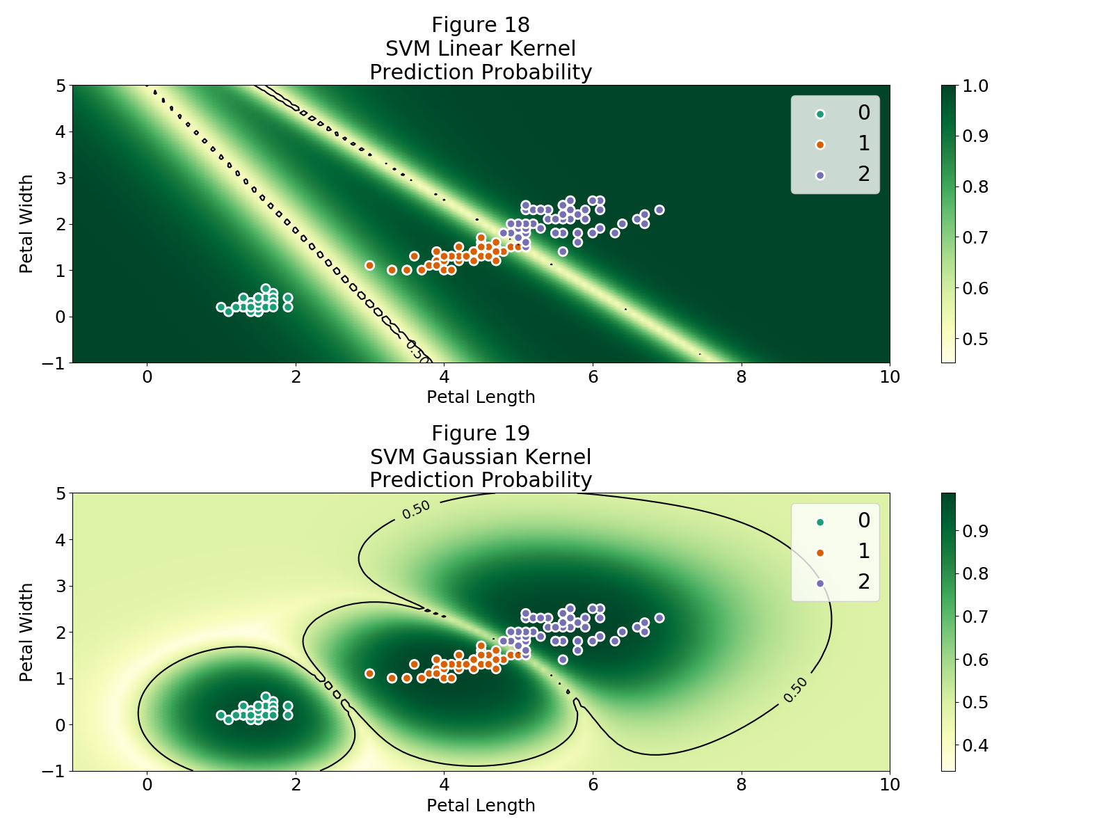
Figure 18 shows that the SVM with the linear kernel also suffers from the issues discussed. In general any discriminative model that is trying to model the conditional probability via some transformation of the dot product $\Theta\cdot X$ is doomed to be susceptible to adversarial examples attacks.

Figure 19 is beautiful, shows exactly how getting rid of the linearity ($\Theta\cdot X$) allows for non-linear classification boundaries and hence the regions with high probability do not extend indefinitely. In this case all points with high probability are close to our observations, so in principle they should "look" like our observations.

A SVM with a Gaussian kernel can't accomplish the extremely complicated tasks that deep neural networks can, but an idea could be to find a way to implement a non-linear kernel between the last hidden layer and the output layer. This discussion is outside the of scope of this article, but hopefully I will find the time to look into it and write about my findings.

Another solution to the above discussed issues lies in a completely different perspective, instead of trying to model the conditional probability, try to model the joint probability with generative models. These models should capture the underlying "context" of our observations and not only what makes them different. This fundamental difference allows generative algorithms to do things which are impossible for a DNN. Such as producing never seen examples which have a striking resemblance to original observations, and even more to tune the context of these examples. A super nice demonstration is the generation of never seen faces where the degree of smiling and sunglasses is tuned.

Adios

Well that took much more work than I expected. I hope you enjoyed reading this blog post and got excited about deep learning.

You can find the code here.

If you have any other questions just ping me in twitter @rragundez.